Note: This is part 3 of Financial Intelligence Data Platform series. you could see the previous part here:

Part 1: Building ETL pipeline from Scratch

Part 2: First Cloud Migration

Good day. Readers,

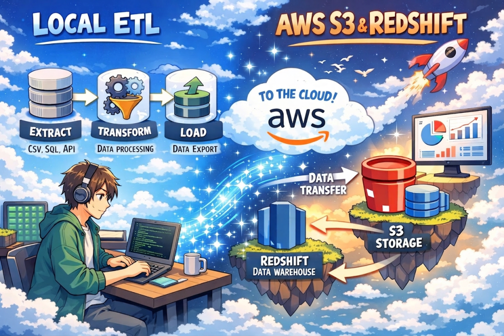
After we successfully migrated our local ETL pipeline to the Cloud infrastructure in Part 2, in this part, we leverage the pipeline with 3 industrial standard tools: Apache Airflow as an automatic pipeline orchestration tool instead of manual execution like the previous part, dbt (Data Build Tool), which organizes the loaded data from the lake to a user-ready data mart, and GitHub Actions, which automates the testing process for every push to remote repository.

Project Architecture

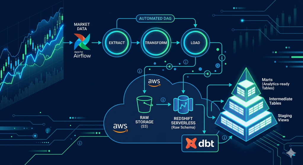
The key distinction from Part 2: Airflow replaces the manual pipeline.py run with a DAG that passes state between tasks via XCom and handles failures with automatic retries and callbacks. dbt then picks up from the raw Redshift tables and produces analytics-ready mart tables through three clean transformation layers — all version-controlled in SQL.

Tech Stack, Prerequisites, and Project Structure

Tech Stacks

In addition to the cloud infrastructure from Part 2, we add the orchestration tools (Airflow), data transformation tools (dbt), and automated CI/CD pipeline (GitHub Actions ) onto our project, so the tech stacks so far would look like this:

Layer	Tools used
Language	Python 3.9+
Orchestration	Apache Airflow 2.9 (via Docker)
Transformation	dbt-redshift 1.10
SQL Linting	sqlfluff
Local Database	PostgreSQL 15
Cloud Database	Amazon Redshift Serverless
Cloud Storage	Amazon S3
AWS SDK	boto3
Local DB Driver	psycopg2-binary
Cloud DB Driver	redshift-connector
DB Toolkit	SQL Alchemy
Data processing	pandas, numpy
HTTP	requests
System Configuration	python-ditenv
Containerisation	Docker
Testing	pytest, moto
CI/CD	GitHub Actions

Prerequisites

From the prerequisites mentioned in Part 2, in this part, we need to install the containerized version of Apache Airflow, dbt, and sqlfluff. We could install the dbt in and sqlfluff now with the following command, since we could install it directly into our virtual environment. However, we will exaplain how to install the Airflow container later in this article.

			
``` PowerShell Terminal
pip install dbt-redshift sqlfluff
pip freeze > requirements.txt

Project Structure

			
finance_data_platform/
├── .github/
│   └── workflows/
│       └── ci.yml                  # CI: pytest, dbt parse, dbt test staging, sqlfluff, DAG integrity
│
├── airflow/
│   ├── docker-compose.yaml         # Official Airflow Docker Compose stack
│   ├── dags/
│   │   └── stock_pipeline_dag.py   # Scheduled DAG: extract >> transform >> load (Mon–Fri 23:00)
│   ├── config/
│   ├── logs/
│   └── plugins/
│
├── finance_dbt/
│   ├── dbt_project.yml             # dbt project config
│   ├── .sqlfluff                   # sqlfluff config: jinja templater, redshift dialect
│   ├── models/
│   │   ├── staging/                # stg_stock_prices, stg_company_metadata (views)
│   │   │   ├── sources.yml         # Declares raw Redshift tables as dbt sources
│   │   │   └── schema.yml          # Column docs + generic tests
│   │   ├── intermediate/           # int_stock_prices_enriched (table)
│   │   └── marts/                  # mart_daily_stock_performance (incremental), mart_sector_volume_summary (table)
│   ├── tests/                      # Singular SQL tests
│   │   ├── assert_no_negative_prices.sql
│   │   ├── assert_volume_gt_zero.sql
│   │   ├── assert_high_gte_low.sql
│   │   └── assert_cumulative_return_base.sql
│   └── sqlfluff_macros/            # Mock Jinja macros for sqlfluff (outside dbt macro path)
│       └── sqlfluff_mocks.sql
│
├── profiles.yml                    # dbt connection profiles (reads from env vars — no secrets)
├── src/                            # (same as Part 2 — unchanged)
└── tests/
    ├── conftest.py
    ├── test_transform.py
    ├── test_loaders.py
    ├── test_s3_client.py
    └── test_dag_integrity.py       # NEW: Airflow DagBag import + structure validation

		

How to:

Set up Apache Airflow

Start Airflow with Docker Compose

As Airflow doesn’t support direct installation on Windows machines, we need to do a workaround by installing it as a Docker container instead of installing it directly on the OS. Fortunately, this approach gives us the OS-neutral advantage.

First, we need to create a new airflow folder to store its services (scheduler, webserver, worker, redis, postgres, triggerer, etc.) and configuration without conflicts with our current project settings. We use the following terminal commands to install an Airflow as a container.

			
``` PowerShell Terminal
# in our root folder, create the new file
mkdir airflow
# in our newly created folder, download the .yaml file of Airflow from the sources
cd airflow
curl -LfO 'https://airflow.apache.org/docs/apache-airflow/2.9.3/docker-compose.yml'
# create the new folder inside airflow folder and .env file
mkdir -p dags logs plugins config
echo -e "AIRFLOW_UID=$(id -u)" > .env
# in case of creating projects in Windows machine, use UID=50000 instead
echo -e "AIRFLOW_UID=50000" > .env

		

Then, copy the content from environment variables (.env) file from the root folder into the newly created one within the airflow folder. Airflow will use these variables for further actions.

Then, we will initialize the airflow container using the following command:

			
``` PowerShell Terminal
docker compose up airflow-init   # one-time DB migration + admin user creation
docker compose up -d             # starts all services in background

From this point, we could verify our installation so far by accessing your local port 8080 (via http://localhost:8080) in your web browser. If you could see Airflow web UI and be able to login using the username=airflow and password=airflow. You’re good to go.

Configure Airflow Connections

In Airflow UI, you need to configure your S3 and Redshift connections by going to Admin → Connections, then create these two connections

AWS S3 (aws_default):

Field	Value
Connection Type	Amazon Web Services
AWS Access Key ID	<Access key from .env>
AWS Secret Access Key	<Secret key from .env>
Extra	{‘region_name”: “your-s3-region”}

Redshift (redshift_default):

Field	Value
Connection Type	Amazon Redshift
Host	<Redshift_host from .env>
Schema	finance_db
Loging	<Redshift_user from .env>
Password	<Redshift_password from .env>
Port	5439

Build the DAG

This part could also be called the Orchestration migration, as we’re gonna change our manual orchestration script into a DAG (Direct Acyclic Graph), which would be executed automatically by Airflow. To minimize the change to the current workflow due to this change, we would wrap our methods used in each of our current phases of orchestration into a new method that represents each phase, then initialize the instance of DAG to orchestrate them together.

You could see the full method structure of the file in our GitHub repository. Here is just a quick illustration of the detailed extraction process to show how things work together.

			
``` ./airflow/dags/stock_pipeline_dag.py
from datetime import datetime, timedelta
import logging
from airflow import DAG
from airflow.operators.python import PythonOperator
symbols = ['TICK1', 'TICK2', 'TICK3']
# extraction method
def extract_task(**context):
  """Fetch raw data from API"""
  import time
  from src.extract.alphavantage_ingest import fetch_stock_prices, fetch_company_metadata
  # declare the blank results, we will forward them to next ETL phase
  results = {}
  # through each tick, we extract the data using our existing fetching function. Then, append onto the results
  for symbol in symbols:
    filepath = fetch_stock_prices(symbol)
    time.sleep(12) # use 12 secs to avoid API request limit (5 req per minute for free tier AlphaVantage users)
    metadata_filepath = fetch_company_metadata(symbol)
    time.sleep(12)
    # append the fetch output to the results
    results[symbol] = {
      "prices": filepath,
      "metadata": metadata_filepath
    }
  # push the results via XCom mechanism to the transformation phase
  context["ti"].xcom_push(key="filepaths", value=results)
# transformation method
def transform_task(**context):
  filepaths = context["ti"].xcom_pull(key="filepaths", task_ids="extract")
  transformed = {}
  ### ... transformation process ... ###
  context["ti"].xcom_push(key="transformed", value=transformed)
# loading method
def load_task(**context):
  transformed = context["ti"].xcom_pull(key="transformed", task_ids="transform")
  ### ... loading process ... ###
# default arguments to configure the DAG
default_args = {
  "owner": "airflow",
  "retries": 3,
  "rety_delay": timedelta(minutes=10),
  "on_failure_callback": notify_on_failure
}
# DAG (putting them altogether)
with DAG(
  dag_id = "stock_pipeline_dag",
  default_args = default_args,
  start_date = datetime(2026,5,1),
  schedule_interval = "0 23 * * 1-5",
  catchup=False,
  sla_miss_callback = sla_miss_callback
) as dag:
  extract = PythonOperator(
    task_id = "extract",
    python_callable = extract_task,
    sla=timedelta(hours=1)
  )
  transform = PythonOperator(
    task_id = "transform",
    python_callable = transfrm_task,
    sla=timedelta(hours=1, minutes=30)
  )
  load = PythonOperator(
    task_id = "load",
    python_callable = load_task,
    sla=timedelta(hours=2)
  )
  # define task dependencies (show how those are orchestrated altogether)
  extrat >> transform >> load

		

You could see that we implement XCom mechanism between ETL phase. This strategy has its own benefits over saving each phase’s outputs as intermediate files or saving the output as a Python variable. First, Airflow DAG deletes all shared in-memory variables unless we squeeze all these ETL tasks into one, which is not ideal for separated tasks architecture. Moreover, saving the output as intermediate files exposes the pipeline outside the managed DAG, which is prone to failure if the intermediate files are shuffled.

You could see the argument called sla or callback in our DAG components. SLA stands for ‘Service Level Agreement’. In this case, for example, we define the extract node to run and retries for the defined number of times shown in default_args. Then, if Airflow orchestration gets stuck on this phase for an hour, we could consider that this node misses the SLA. We will place the notification mechanism to handle this one. We call this mechanism SLA monitoring.

Task Callbacks and SLA Monitoring

To add guardrails to handle the pipeline failure. We would add the SLA monitoring to let users (system administrator, in this case) know which orchestration node fails. In this case, we will add 2 new methods onto our DAG; sla_miss_callback() and notify_on_failure() method. We could see it in our DAG script as follows:

			
``` ./airflow/dags/stock_pipeline_dag.py
def notify_on_failure(context):
    """Called when any task fails. Wire to Slack or email in production."""
    task_instance = context["task_instance"]
    logger.error(
        f"Task FAILED: DAG={task_instance.dag_id}, "
        f"Task={task_instance.task_id}, "
        f"Run={context['run_id']}"
    )
    # area to add SlackWebhookOperator or EmailOperator to send notification on failure
def sla_miss_callback(dag, task_list, blocking_task_list, slas, blocking_tis):
    """Fires when a task exceeds its SLA window. Useful for alerting on performance issues."""
    logger.warning(
        f"SLA MISSED on DAG '{dag.dag_id}'."
        f"MIssed tasks: {[str(t) for t in task_list]}"
    )
    # area to add SlackWebhookOperator or EmailOperator to send notification on failure

		

We could also tell which channel DAG fails could notify users; Airflow supports notifications through Slack (SlackWebhookOperator) or an email (EmailOperator), but our project doesn’t cover these.

Configuration on `airflow/docker-compose.yaml`

From this point, we expected that our built DAG would appear in Airflow UI. Unfortunately, we need some adjustments to docker-compose.yaml to make the DAG runs as expected in this project.

Adding Environment Variables

We need to map the .env variables into docker-compose.yml to let the airflow container include those variables into the DAG. To do so, go to x-airflow-common → environment section. Then add these .env variables to the environment.

			
``` ./airflow/docker-compose.yaml
x-airflow-common:
  environment:
    # add .env variables to the environment
    DB_ENGINE: ${DB_ENGINE:-}
    
    AWS_REGION: ${AWS_REGION:-}
    AWS_ACCESS_KEY: ${AWS_ACCESS_KEY:-}
    AWS_SECRET_KEY: ${AWS_SECRET_KEY:-}
    S3_BUCKET_NAME: ${S3_BUCKET_NAME:-}
    REDSHIFT_HOST: ${REDSHIFT_HOST:-}
    REDSHIFT_PORT: ${REDSHIFT_PORT:-}
    REDSHIFT_NAME: ${REDSHIFT_NAME:-}
    REDSHIFT_USER: ${REDSHIFT_USER:-}
    REDSHIFT_PASSWORD: ${REDSHIFT_PASSWORD:-}
    REDSHIFT_IAM_ROLE: ${REDSHIFT_IAM_ROLE:-}
    ALPHAVANTAGE_API_KEY: ${ALPHAVANTAGE_API_KEY:-}
  user: "${AIRFLOW_UID:-50000}:0"

		

Define DAG resources filepath and volumes

In accordance with our project structure, we built the Airflow components in ./airflow folder while the resources, including a set of ETL methods, are located in ./src, so we need to declare this resource path to the Airflow container.

			
``` ./airflow/docker-compose.yaml
x-airflow-common:
  environment:
    PYTHONPATH: /opt/airflow:/opt/airflow/src
  volumes:
    - ../src:/opt/airflow/src

		

Remove DAG Examples

While this is not a mandatory fix, removing the irrelevant example DAGs makes our Airflow UI much cleaner. You could adjust this variable:

			
``` ./airflow/docker-compose.yaml
x-airflow-common:
  environments:
    AIRFLOW__CORE__LOAD_EXAMPLES: 'false'

After all, you need to restart the Docker container by

			
``` PowerShell Terminal
docker-compose down
docker-compose up -d

Then, when you access Airflow UI once again, you’ll see your DAG. Trigger the DAG to see if these nodes run properly.

Also, don’t forget to add the integer 5439 in Redshift port connection ./src/db-connect.py to prevent potent errors from machien read the integer as strings

			
``` ./src/db_connect.py
# leave other components as it is, just add the port as an integer
def db_connect():
  engine = os.getenv("DB_ENGINE", "postgres")
  if engine == "redshift":
    conn = redshift_connector.connect(
      port = int(os.getenv("REDSHIFT_PORT"), 5439)
      # ... leave other connection parameter as it is ...
    )
  

		

Set up dbt

dbt (Data Build Tool) is a tool primarily invented to transform the data in ELT process. It manages data loaded into SQL database, then transforms and produces the clean, documented, and tested analytics tables, a.k.a Data Mart.

After install dbt-redshift as shown in prerequisite section, you could initialize the dbt projects under our root path by:

			
``` PowerShell Terminal
dbt init finance_dbt

If doing it right, dbt will let you select the adapter. We need you to choose redshift for this project. Then dbt will creates the dbt project folder called finance_dbt under our project root.

Configure `profiles.yml`

dbt also creates another file outside the project folder called profiles.yml, which contains the environment variables. However, to avoid exposing environment variables outside .env files. We would create ~/.dbt/profiles.yml to let dbt loads the environment variables for further usage.

			
``` ~/.dbt/profiles.yml (the outside the project)
finance_dbt:
  outputs:
    dev:
      host: "{{ env_var('REDSHIFT_HOST') }}"
      port: 5439
      dbname: "{{ env_var('REDSHIFT_NAME') }}"
      user: "{{ env_var('REDSHIFT_USER') }}"
      password: "{{ env_var('REDSHIFT_PASSWORD') }}"
      schema: analytics
      threads: 4
      type: redshift
  target: dev

		

This reads the environment variables from ./airflow/.env so we load the variables before running dbt

			
``` PowerShell Terminal
set -a && source airflow/.env && set +a
dbt debug    # should print "All checks passed!"

Then, in./finance_dbt/dbt_project.yml, we need to point our project to this created profile by defining these variables.

			
``` ./finance_dbt/dbt_project.yml
name: 'finance_dbt'
profile: 'finance_dbt'

Define Sources

Before building any model, we declare the raw Redshift tables as sources in ./finance_dbt/models/staging/sources.yml. This is the explicit lineage contract that tells dbt where the data comes from — and allows dbt’s lineage graph to trace all the way back to the raw tables. Here’s the exsample of sources.yml

			
``` ./finance_dbt/models/staging/sources.yml
sources: 
  - name: raw 
    schema: public
    description: "Raw tables loaded by the Airflow pipeline from S3 via Redshift COPY"
    tables:
      - name: stock_prices
        description: "Daily OHLCV stock prices"
        columns:
          - name: symbol
            description: "Ticker symbol"
          - name: date
            description: "Trading date"
          - name: open_price
          - name: high
          - name: low
          - name: close_price
          - name: volume
      - name: dim_metadata
      - name: dim_date

		

From this point forward, all models reference these raw tables with {{ source(‘raw’, ‘table_name’) }} instead of hardcoding schema names.

Build Staging Models

Staging models are then, lightweight views. Their only job is to rename columns, cast typles, and add a loaded_at timestamp — no business logic yet. Here’s how staging models looks like:

			
``` ./finance_dbt/models/staging/stg_stock_prices.sql
{{ config(materialized='view') }}
SELECT
  symbol,
  date,
  open_price,
  high,
  low,
  close_price,
  volume,
  GETDATE() AS loaded_at
FROM {{ source('raw', 'stock_prices') }}

		

			
``` ./finance_dbt/models/staging/stg_company_metadata.sql
{{ config(materialized='view') }}
SELECT
  symbol,
  comapny_name,
  INITCAP(LOWER(sector)) AS sector,
  GETDATE() AS loaded_at
FROM {{ source('raw', 'dim_metadata') }}

		

Notice INITCAP(LOWER(sector)) — this normalises the sector string to title case (e.g., TECHNOLOGY → Technology) at the staging layer, so all downstream models get clean values automatically.

Build Intermediate Models

The intermediate model (int_stock_prices_enriched) is where the analytical joins happen. It joins the two staging views with dim_date, enriching the stock price data with calendar attributes and computing two derived metrics — daily_return and first_close — that the mart models depend on:

			
``` ./finance_dbt/models/intermediate/int_stock_prices_enriched.sql
{{ config(materialized='table') }}
SELECT
  sp.symbol,
  sp.date,
  sp.open_price, sp.high, sp.low, sp.close_price, sp.volume,
  m.company_name,
  m.sector,
  d.day, d.month, d.year, d.quarter, d.day_of_week, d.week_of_year,
  -- daily return: percentabe change from previous close
  ROUND(
    (sp.close_price / LAG(sp.close_price)
      OVER (PARTITION BY sp.symbol ORDER BY sp.date)) - 1, 6
  ) AS daily_return,
  -- anchor close for cumulateive reutnr calculation
  FIRST_VALUE(sp.close_price) OVER (
    PARTITION BY sp.symbol
    ORDER BY sp.date
    ROWS BETWEEN UNBOUNDED PRECEDING AND CURRENT ROW
  ) AS first_close
FROM {{ ref('stg_stock_prices') }} AS sp
LEFT JOIN {{ ref('stg_company_metadata') }} AS m ON sp.symbol = m.symbol
LEFT JOIN {{ source('raw', 'dim_date') }} AS d ON sp.date = d.date

		

This is materialised as a table (not a view) becuase it is joined by two downstream mart models — materialising it once avoids running the join twice.

Built Mart Models

Mart models are the business-facing layer — what an analyst would actually query. We have two.

mart_daily_stock_performance is materialised as incremental, meaning on each dbt run it only appends rows for new dates rather than rebuilding the entire historical table:

			
``` ./finance_dbt/models/mart/mart_daily_stock_performance.sql
{{
  config(
    materialized = 'incremental',
    unique_key = 'symbol_date',
    dist = 'symbol',
    sort = 'date'
  )
}}
SELECT
  symbol || '_' || CAST(date AS VARCHAR) AS symbol_date,
  symbol, date, company_name, sector, close_price, daily_return,
  AVG(close_price) OVER (PARTITION BY symbol ORDER BY date ROWS BETWEEN 4 PRECEDING AND CURRENT ROW) AS sma_5,
  AVG(close_price) OVER (PARTITION BY symbol ORDER BY date ROWS BETWEEN 19 PRECEDING AND CURRENT ROW) AS sma_20,
  STDDEV(daily_return) OVER (PARTITION BY symbol ORDER BY date ROWS BETWEEN 20 PRECEDING AND CURRENT ROW) AS volatility_21,
FROM {{ ref('int_stock_prices_enriched') }}
{% if is_incremental() %}
WHERE date > (SELECT MAX(date) FROM {{ this }})
{% endif %}

		

The {% if is_incremental() %} block is the key: on the first run it builds the full table; on every subsequent run it only inserts rows where date exceeds the current maximum — safe to run daily without duplicating history.

mart_sector_volume_summary aggregates volume and average daily return by sector and date — useful for inter-sector comparisons:

			
``` ./finance_dbt/models/mart/mart_sector_volume_summary.sql
{{ config(materialized='table') }}
SELECT
  sector,
  date,
  SUM(volume) AS total_volume,
  AVG(daily_return) AS avg_daily_return
FROM {{ ref('int_sock_prices_enriched') }}
GROUP BY sector, date
ORDER BY sector, date

		

Add Data Quality Tests

One of dbt’s strongest features is its built-in test framework. We define two types of tests.

Generic tests in schema.yml validate structural rules on every model (not null, uniqueness, referential integrity):

			
``` ./finance_dbt/models/mart/schema.yml
models:
  - name: mart_daily_stock_performance
    columns:
      - name: symbol_date
        tests:
          - not_null
          - unique
      - name: symbol
        tests:
          - not_null
          - relationships:
              to: ref('stg_company_metadata')
              field: symbol

		

Singular tests are custom SQL files that return rows only when the test fails. For example, assert_no_negative_prices.sql:

			
``` ./finance_dbt/models/.../assert_no_negative_prices.sql
SELECT *
FROM {{ ref('stg_stock_prices') }}
WHERE open_price < 0
  OR high < 0
  OR low < 0
  OR close_price < 0

		

If this query returns any rows, the test fails. All four singular tests (assert_no_negative_prices, assert_volume_gt_zero, assert_high_gte_low, assert_cumulative_return_base) run with dbt test.

Here are useful commands to run and test dbt:

			
``` PowerShell Terminal
# move to project's dbt folder
cd finance_dbt
# validate all SQL without a Redshift connection
dbt parse --profiles-dir ..
# build all models
dbt run --profiles-dir ..
# run all data quality tests
run test --profiles-dir ..
# generate and serve the lineage docs
dbt docs generate --profiles-dir ..
dbt docs serve --profiles-dir ..

		

A Note on sqlfluff Mock Macros

One non-obvious design decision: sqlfluff (our SQL linter) needs to resolve Jinja macros like {{ config() }}, {{ ref() }}, and {{ is_incremental() }} before it can line the SQL. we create mock implementations in ./finance_dbt/sqlfluff_macros/sqlfluff_mocks.sql.

The key reason this folder lives outside finance_dbt/macros/ is that dbt scans the macros/ directory at runtime. Placing a mock config() there would override dbt’s internal get_where_subquery macro and silently break dbt test. By puting the mocks in sqlfluff_macros/, sqlfluff finds them but dbty ignores the directory entirely.

Set up CI/CD pipeline

GitHub Actions Workflow

The ./.github/ci.yml pipeline runs on every push and pull request, validating five things in parallel where possible.

			
``` ./.github/ci.yml
jobs:
  test:
    runs-on: ubuntu-latest
    steps:
      - uses: actions/checkout@v3
      - name: Set up Python
        uses: actions/setup-python@v4
        with:
          python-version: '3.9'
      - name: Install dependencies
        run: pip install -r requirements.txt
      - name: Run unit tests
        run: pytest tests/ -m "not integration" --ignore=tests/test_dag_integrity.py -v
      - name: dbt parse (validate SQL)
        run: |
          cd finance_dbt
          dbt parse --profiles-dir ..
      - name: dbt test staging
        run: |
          cd finance_dbt
          dbt test --select staging --profiles-dir ..
      - name: sqlfluff line
        run: sqlfluff line finance_dbt/models/ --dialect redshift
      - name: Airflow DAG integrity
        run: pytest tests/test_dag_integrity.py -v

		

Notice that dbt test --select staging only runs staging-layer tests in CI — these tests run against views (no data needed), so they pass without a live Redshift connection. Full mart tests require actual data and run only locally or in integration environments.

DAG Integrity Testing

test_dag_integrity.py uses Airflow’s DagBag class to verify that the DAG file imports cleanly — no syntax errors, no broken imports, correct task IDs and dependency order:

			
``` ./tests/test_dag_integrity.py
import pytest
from airflow.models import DagBag
def test_dag_bag_loads_without_errors():
    """Ensure all DAGs in the dags/ directory load without import errors."""
    dag_bag = DagBag(dag_folder="airflow/dags", include_examples=False)
    # Fail immediately if any DAG has import errors
    assert dag_bag.import_errors == {}, (
        f"DAG import errors found:\n"
        + "\n".join(f" {path}: {err}" for path, err in dag_bag.import_errors.items())
    )
def test_stock_pipeline_dag_exists():
    """Verify the stoc k pipeline DAG is registered with the correct dag_id."""
    dag_bag = DagBag(dag_folder="airflow/dags", include_examples=False)
    assert "stock_pipeline_dag" in dag_bag.dags
def test_stock_pipeline_dag_structure():
    """Verify the DAG has the expected tasks in the correct order."""
    dag_bag = DagBag(dag_folder="airflow/dags", include_examples=False)
    dag = dag_bag.dags["stock_pipeline_dag"]
    task_ids = set(dag.task_ids)
    assert task_ids == {"extract", "transform", "load"}
    # Verify dependency chain: extract >> transform >> load
    extract = dag.get_task("extract")
    assert "transform" in [t.task_id for t in extract.downstream_list]
    transform = dag.get_task("transform")
    assert "load" in [t.task_id for t in transform.downstream_list]

		

This means if anyone accidentally breaks an import in the DAG file, CI catches it before it ever reaches the Airflow scheduler in production.

Conclusion

Stage 3 transforms a manually triggered cloud pipeline into a fully automated, observable, and documented data platform. Specifically, we covered:

Airflow DAG orchestration: replacing python -m src.pipeline with a scheduled extract >> transform >> load DAG, with XCom-based state sharing between tasks, per-task SLA windows, automatic retries, and failure callbacks ready for Slack or email integration.
dbt transformation layers: three clean SQL layers (staging views →enriched intermediate table → incremental mart tables) with full column-level documentation, generic tests, and custom singular SQL tests — all version-controlled alongside the rest of the codebase.
Incremental materialisation: mart_daily_stock_performance appends only new rows on each run using is_incremental(), avoiding a full historical rebuild every day.
CI/CD pipeline: GitHub Actions validates unit tests, dbt SQL syntax, staging-layer data quality tests, SQL linting, and DAG import integrity on every push
sqlfluff mock macros: an intentional architectural decision to keep Jinja mock macros outside the macros/ directory, preventing them from interfering with dbt’s internal macro resolution during dbt_test.

Honestly, the most valuable lesson from this stage is how these two tools complement each other. Airflow is the when and how reliably — it ensures the pipeline runs on schedule and recovers from failures. dbt is the what it means — it gives the raw Redshift data a clean, tested, documented shape that analysts can actually trust.

In the next part, we will bring Apache Spark into the platform, rewriting the analytics computations as distributed PySpark jobs that read from S3 and write results back as Delta Lake tables on Databricks.

Stay tuned — and as always, the full code is available in the GitHub repository.

Nextstep Analytics

Financial Intelligence Data Platform (Part 3) – Automatic Orchestration, Transformation, and CI/CD pipeline

Project Architecture

Tech Stack, Prerequisites, and Project Structure

Tech Stacks

Prerequisites

Project Structure

How to:

Set up Apache Airflow

Start Airflow with Docker Compose

Configure Airflow Connections

Build the DAG

Task Callbacks and SLA Monitoring

Configuration on `airflow/docker-compose.yaml`

Set up dbt

Configure `profiles.yml`

Define Sources

Build Staging Models

Build Intermediate Models

Built Mart Models

Add Data Quality Tests

A Note on sqlfluff Mock Macros

Set up CI/CD pipeline

GitHub Actions Workflow

DAG Integrity Testing

Conclusion

Leave a comment Cancel reply

“Hello World :)”

Subscribe to our site here.

Meet me at

Recent posts

Financial Intelligence Data Platform (Part 3) – Automatic Orchestration, Transformation, and CI/CD pipeline

Financial Intelligence Data Platform (Part 1) – Building ETL Pipeline from Scratch

World Tourism: from Data Pipeline to Analysis

Division of Virginia: Data Analysis

Data analysis and predictions of Diabetes

Project Architecture

Tech Stack, Prerequisites, and Project Structure

Tech Stacks

Prerequisites

Project Structure

How to:

Set up Apache Airflow

Start Airflow with Docker Compose

Configure Airflow Connections

Build the DAG

Task Callbacks and SLA Monitoring

Configuration on airflow/docker-compose.yaml

Set up dbt

Configure profiles.yml

Define Sources

Build Staging Models

Build Intermediate Models

Built Mart Models

Add Data Quality Tests

A Note on sqlfluff Mock Macros

Set up CI/CD pipeline

GitHub Actions Workflow

DAG Integrity Testing

Conclusion

Share this:

Leave a comment Cancel reply

“Hello World :)”

Subscribe to our site here.

Meet me at

Recent posts

Configuration on `airflow/docker-compose.yaml`

Configure `profiles.yml`