Note: This is part 2 of Financial Intelligence Data Platform series, see the previous part here
Good Day, Readers,
After we initially built the ETL pipeline from scratch, in this part, we will migrate the data storage and database into cloud infrastructures. Ensure that we don’t lose the data in case the local machine crashes.
- Project Architecture
- Tech Stack, Prerequisites, and Project Structures
- How to:
- Conclusion
Project Architecture
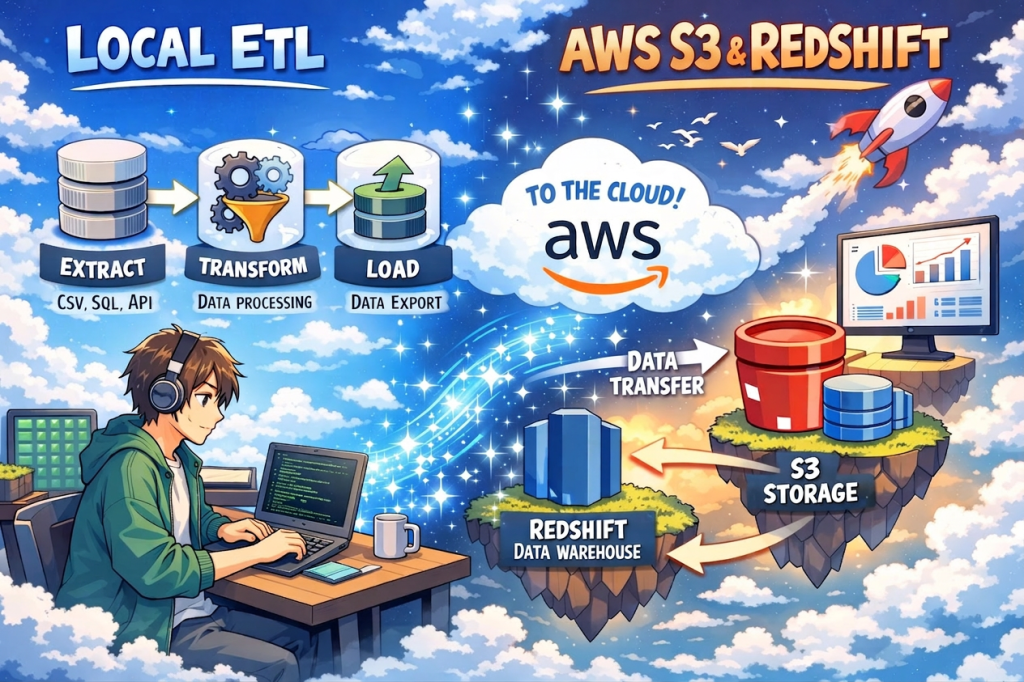
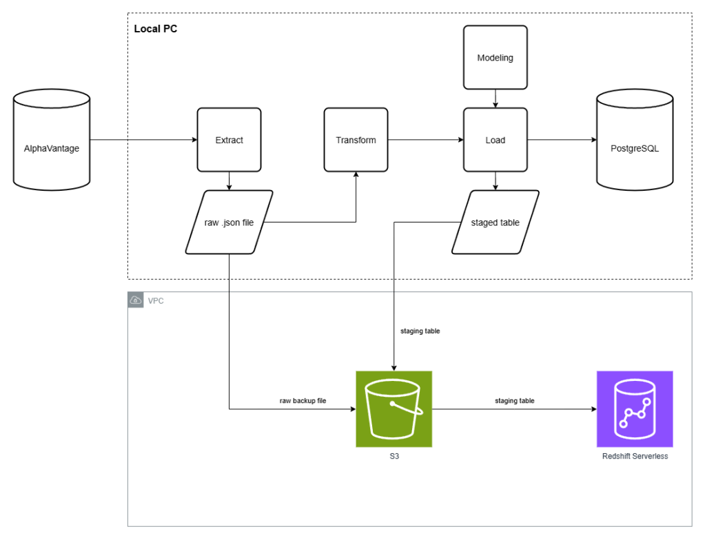
From our ETL pipeline, which runs locally in the previous part, this one will adopt the capabilities of AWS S3 as a cloud storage for raw data and a staging table (processed data ready to write into a database) area. Then, Redshift Serverless would access that staged table and write the data into the database.
Tech Stack, Prerequisites, and Project Structures
Tech Stacks
In addition to the local version of ETL pipelines, we need to add some cloud-related tools to our pipeline as shown in the complete list below
| Layer | Tools used |
| Language | Python 3.9+ |
| Local Database | PostgreSQL 15 |
| Cloud Database | Amazon Redshift Serverless |
| Cloud Storage | Amazon S3 |
| AWS SDK | boto3 |
| Local DB Driver | psycopg2-binary |
| Cloud DB Driver | redshift-connector |
| DB Toolkit | SQLAlchemy |
| Data processing | pandas, numpy |
| HTTP | requests |
| System Configuration | python-dotenv |
| Containerisation | Docker |
| Testing | pytest, moto |
Prerequisites
Besides Python 3.9, Docker Desktop, and AlphaVantageAPI, which we have mentioned in the previous part. This part also requires the AWS accounts to work around, as this is one of the developer’s essential tools nowadays. I recommend creating your own AWS account for this project and further use. After creating your new AWS account (also known as the root account), it’s strongly recommended to
- Enable MFA (Multi-Factor Authentication) to more prevent unauthorized login. You could use MFA method of your choice e.g. Google Authentication app.
- After logging into AWS management console, go to IAM → Users → Create user. Then create a new user with access to AWS management console, create the password, then create the user. With that, you’ve already got the new administrator account that would handle almost all tasks like what root users do. This is to avoid exposing root users to others.
From now on, we will use admin users to manage our AWS infrastructure.
Project Structure
finance_data_platform/├── docker-compose.yml # PostgreSQL container for local mode├── requirements.txt # All dependencies├── .env # Environment variable template│├── sql/│ ├── sma.sql # SMA5 and SMA20 window functions│ ├── daily_returns.sql # Daily return calculation│ ├── volatility.sql # 21-day rolling volatility (stddev of returns)│ └── cumulative_return.sql # Cumulative return from earliest date│├── data/│ ├── raw/{symbol}/ # Raw JSON responses from AlphaVantage│ └── analytics/ # CSV output of SQL analytics queries│├── src/│ ├── db_connect.py # Connection factory — postgres or redshift via DB_ENGINE env flag│ ├── pipeline.py # Main ETL orchestration (fetch → S3 → transform → load)│ ├── reprocess_pipeline.py # Reprocess from local/S3 files without API calls│ ├── analytics.py # Execute SQL analytics queries; export to CSV│ ││ ├── extract/│ │ └── alphavantage_ingest.py # API fetch with rate-limit retry, quota detection, dual-write to S3│ ││ ├── storage/│ │ └── s3_client.py # boto3 wrapper: upload_file, list_objects, download_file│ ││ ├── transform/│ │ └── transform_stock.py # OHLCV + calendar attribute derivation; metadata parsing│ ││ ├── load/│ │ ├── dimension_loader.py # dim_date and dim_metadata — Postgres ON CONFLICT / Redshift DELETE+INSERT│ │ ├── fact_loader.py # stock_prices — Postgres bulk insert / Redshift S3 COPY + DELETE+INSERT│ │ └── redshift_copy_loader.py # COPY from S3 into staging tables; VACUUM+ANALYZE post-load│ ││ └── modeling/│ ├── create_dimension_tables.py # PostgreSQL dimension table DDL│ ├── create_fact_tables.py # PostgreSQL fact table DDL│ ├── create_indexes.py # PostgreSQL performance indexes│ └── create_redshift_schema.py # Redshift DDL — DISTKEY/SORTKEY/ENCODE + staging tables│└── tests/ ├── conftest.py # db_cursor fixture — isolated TEMP tables, auto-rollback ├── test_transform.py # Unit tests for transformation logic ├── test_loaders.py # Integration tests for all loaders (dim + fact) └── test_s3_client.py # Unit tests for S3 wrapper using moto (no real AWS)
How to:
Configure your Environment
Configure Project Dependencies
In this project, you need to add the new dependencies using the following scripts in your terminal:
cd your-project-directorypip install boto3 redshift_connector awscli moto[s3]==5.1.2pip freeze > requirements.txt
Configure Project Environment Variables
Then, you also need to add new variables to your .env file. We will guide you on how to configure each of them along the way, but it’s supposed to look something like this one at the end of this phase.
# AlphaVantage API configurationALPHAVANTAGE_API_KEY=<your_api_key># database configurationDB_HOST=localhostDB_PORT=5432DB_NAME=finance_dbDB_USER=<your_finance_user>DB_PASSWORD=<your_finance_password># AWS credentialsAWS_REGION=us-east-1AWS_ACCESS_KEY=<your_aws_access_key>AWS_SECRET_KEY=<your_aws_secret_access_key># S3 configurationS3_BUCKET_NAME=<your_s3_bucket_name># Redshift serverless configurationREDSHIFT_HOST=<your_redshift_workgroup_name>.<your_aws_account_id>.<your_aws_region>.redshift-serverless.amazonaws.comREDSHIFT_PORT=5439REDSHIFT_NAME=finance_dbREDSHIFT_USER=<your_redshift_user>REDSHIFT_PASSWORD=<your_redshift_password>REDSHIFT_IAM_ROLE=arn:aws:iam::<your_aws_account_id>:role/<your_custom_RedshiftS3ReadRole># default database engineDB_ENGINE=redshift
Configure Database Connection
To make sure that our pipeline could pick the correct variable while connect to the database, we need to define which variables they need to pick. Here, ./src/db_connect.py, would handle this task.
import psycopg2import osfrom dotenv import load_dotenvimport redshift_connectorload_dotenv()def db_connect(): engine = os.getenv("DB_ENGINE", "postgres") if engine == "redshift": conn = redshift_connector.connect( host = os.getenv("REDSHIFT_HOST"), port = os.getenv("REDSHIFT_PORT"), database = os.getenv("REDSHIFT_NAME"), user = os.getenv("REDSHIFT_USER"), password = os.getenv("REDSHIFT_PASSWORD") ) else: conn = psycopg2.connect( host = os.getenv("DB_HOST"), port = os.getenv("DB_PORT"), dbname = os.getenv("DB_NAME"), user = os.getenv("DB_USER"), password = os.getenv("DB_PASSWORD") ) return conn
Configure the AWS components
Simple Storage Services (S3)
finance-data-platform-raw bucket
First, go to S3 services (you could do that by searching). Then, create the new bucket with versioning-enabled named finance-data-platform-raw. The bucket from our project would follow this structure.
finance-data-platform-raw/├── {symbol}/│ ├── {symbol}_{YYYY-MM-DD}.json # OHLCV data│ ├── {symbol}_metadata.json # metadata...
We will use this S3 bucket to store raw, extracted data in .json format.
boto3 wrapper
After we have done the IAM configuration (please see below), we create ./storage/s3_client.py in our local directory. We will use this to contain the utility function regarding the S3 bucket; create a client, upload the file, list objects in the bucket, and download the file.
IAM
In this project, we have to create the following IAM instances:
FinancePipelineS3Policy
Go to IAM (you could do that by search) → Policies → Create policy. You could either create the new policy by one of these methods;
- Visual policy editor: You would associate the policy with S3 services, then mount the action of the
PutObject,GetObject, andListBicketto the policy, then mount into our created S3 bucket (finance-data-platform-raw) as an associated resource. - JSON policy editor: You could configure the policy identically using JSON. Use the following JSON code in our policy editor.
{ "Version": "2012-10-17", "Statement": [ { "Sid": "VisualEditor0", "Effect": "Allow", "Action": [ "s3:PutObject", "s3:GetObject", "s3:ListBucket" ], "Resource": [ "arn:aws:s3:::finance-data-platform-raw", "arn:aws:s3:::finance-data-platform-raw/*" ] } ]}
finance-pipeline-local User
Then, go to IAM → Users → Create user. Create a new user called finance-pipeline-local without access to the AWS management console. Then, mount the created FinancePipelineS3Policy directly onto this user, so it has the permissions as allowed accordingly.
After creating the user, go to IAM → Users, then select the user. Then, go to Security Credentials → Create access key for Local code use case. Then you get the access key with its secrets (it will show you only once. You need to create a new one in case that you lost it). We will store it in .env file under the variable called AWS_ACCESS_KEY and AWS_SECRET_KEY, respectively.
RedshiftS3ReadOnlyPolicy
Besides the Policy and User regarding S3, we need to create another policy and role to be attached to AWS Redshift. Here we create another role, RedshiftS3ReadOnlyPolicy, shown as follows:
{ "Version": "2012-10-17", "Statement": [ { "Sid": "VisualEditor0", "Effect": "Allow", "Action": [ "s3:GetObject", "s3:ListBucket" ], "Resource": [ "arn:aws:s3:::finance-data-platform-raw/*", "arn:aws:s3:::finance-data-platform-raw" ] } ]}
You could see that this is the FinancePipelineS3Policy, but without s3:PutObject permissions. As the Redshift instance doesn’t need to update (Put) the raw extracted data from the AlphaVantage API, this new role is created to comply with Least-Privilege concepts.
RedshiftS3ReadRole
Then, we create the new Role, which would be attached to the created policy. Go to IAM → Roles → Create role. Then, create the new role with the following configurations:
- Trusted Entity Type: AWS service
- Use case: Redshift → Redshift – Customizable
- Permission Policies:
RedshiftS3ReadOnlyPolicy - Role name:
RedshiftS3ReadRole
After creating the role, we collect the role’s ARN string, then collect it in .env file, called REDSHIFT_IAM_ROLE.
Security Groups
Then, we create the new security groups to grant inbound traffic from the local machine into the Redshift serverless instance. We search for Security Groups in the search bar (it must be under the EC2 services). Then, create the new security groups called finance-data-redshift-sg, which associated the inbound rules connection to TCP port 5439 from your current IP address (Note: In case you need to do this project remotely, consider either using a VPN to your home location, or changing your inbound IP address temporarily.
Redshift Serverless
Why Redshift Serverless?
Before we go further into Redshift configuration, this question might come right to your mind. Generally speaking, instead of spending hundreds of dollars a month to use the server version of Redshift, serverless architecture could help us save the cost for this project, as AWS charges us a fee based on the queries used in our project, which could cost around $5 – 10 a month. Here’s how we do it.
Provision Redshift Serverless via AWS console. Go to Redshift services → create a Redshift serverless instance. The wizard is split into namespace and workgroup configuration.
Namespace setup (finance-data-platform)
Although there is default settings available for a new Redshift instance, we need to create a new one with customized settings. Then, the wizard prompts for an admin username and password. You could define your own username and password here. We’re gonna use it for further Redshift Access as Redshift creates this user as a super user in the created database. Then, save them as REDSHIFT_USER and REDSHIFT_PASSWORD in the .env file. Then, attach your created RedshiftS3ReadRole to the namespace here under the field Associate IAM roles.
Workgroup setup (finance-data-db)
Then, associate the workgroup with your VPC (Virtual Private Cloud — don’t worry, AWS will use the existing one, or create a new in case that you don’t have one yet) and created security groups (finance-data-redhsift-sg). Then, set the base capacity for processing the data warehouse workloads at 8 RPUs (Redshift Processing Unit) as a suitable size for the project.
Then, the endpoint could be obtained from workgroup configuration → workgroup created → endpoint section.
Then, go to the workgroup configuration → edit → enable Publicly Accessible to allow inbound connections from outside of AWS network, which is the local pipeline in our case.
Next, open Redshift Query Editor v2 (search the service, or go to Redshift → Query data → Query in query editor v2). The Redshift Serverless instance appears in the left pane. For the first-time connection, click it and choose Temporary credentials (federated user) with a database called dev. This uses your current AWS Console IAM identity. Then create finance_db by running in the right panel:
CREATE DATABASE finance_db;
Secrets Manager
After finance_db exists, set up a saved connection for repeated Query Editor v2 use: add a new connection, choose AWS Secrets Manager as the authentication method, then fill in the following variables and their values.
- Secret name: as defined
- host:
your_redshift_endpoint - port: 5439
- engine:
redshift
The wizard creates the secret in AWS Secrets Manager automatically. Please note that this secret will be called during Query Editor UI access. While our local ETL pipeline will access the database using credentials stored in .env file. We will show you how to integrate those credentials into our pipeline later in this article.
Update your ETL pipelines
Extract
In src/extract/alphavantage_ingest.py, Besides of downloading the raw data then save it as .json files in the local machine as described in the previous part. In the meantime, we’re gonna upload the raw data into the created S3 bucket in the meantime for both OHLCV and the company’s metadata as well. We called it “Dual-write” systems.
Transform
Basically, we don’t have to modify the transform process that we’ve made from our last part. However, we’ve encountered some errors with Redshift’s reserved keywords like open and close, which needs some fixes. We’re gonna delve into this matter, then.
Modeling
As we’re going to build our new cloud-based database (Redshift serverless), we need to create the new schema for the Redshift database as well. Due to the difference in storage architecture between PostgreSQL, which we use locally, and Redshift, they need different DDL (Data Definition Language) in data modelling
Key differences between Redshift and PostgreSQL DDL:
- No FOREIGN KEY: Redshift supports the syntax to prevent crashes, but ignores them at runtime.
- No PRIMARY KEY enforcement: Redshift treats primary key as a hint for the query planner, but not as a hard constraint. However, we still need to keep them unique and hint the Redshift using
DISTKEY.- DISTSTYLE ALL on dimension tables: As Redshift is built on a distributed database architecture, it means a table in a database is physically split across multiple compute nodes, each with its own CPU, memory, and storage. Make it possible to process large datasets much faster than a single-node PostgreSQL. DISTSTYLE ALL means it copies the entire selected table to all nodes, reducing the compute time when querying inter-table operations such as JOIN.
- No CREATE INDEX: It is not supported by Redshift.
You could see the GitHub repository for the detailed version of our scheme there. Here is an example of the difference in the data model between PostgreSQL and Redshift:
// PostgreSQLCREATE TABLE IF NOT EXISTS stock_prices ( symbol TEXT, date DATE, open_price NUMERIC, high NUMERIC, low NUMERIC, close_price NUMERIC, volume BIGINT, PRIMARY KEY (symbol, date), FOREIGN KEY (symbol) REFERENCES dim_metadata(symbol), FOREIGN KEY (date) REFERENCES dim_date(date));
// RedshiftCREATE TABLE IF NOT EXISTS stock_prices ( symbol VARCHAR(20) NOT NULL ENCODE lzo, date DATE NOT NULL ENCODE az64, open_price NUMERIC(12,4) ENCODE az64, high NUMERIC(12,4) ENCODE az64, low NUMERIC(12,4) ENCODE az64, close_price NUMERIC(12,4) ENCODE az64, volume BIGINT ENCODE az64, PRIMARY KEY (symbol, date))DISTKEY (symbol)SORTKEY (date);
This is the difference between the data model of OHLCV table. You could see that we have no more FOREIGN KEY definitions in Redshift. Moreover, we hint at the primary key using the combination of symbol and date with the keyword DISTKEY() and SORTKEY(), respectively.
Load
Compared to other ETL processes, our cloud migration affects the loading stage the most. Here is what the loading phase in ETL pipelines does regarding our AWS cloud-based architecture.
Here, we encounter another architecture difference between local PostgreSQL and Redshift. Unlike INSERT ... ON CONFLICT DO NOTHING that we’re familiar with in PostgreSQL, Redshift doesn’t support ON CONFLICT. So, it won’t reject the duplicates. Moreover, instead of slower row-by-row writing with INSERT, we implement bulk load style COPY into our load process.
Therefore, from the single INSERT, we need to Serialize → S3 → COPY → DELETE+INSERT → VACUUM+ANALYZE in Redshift. Here are the detailed steps to do so.
Create Utility Function copy_json_from_s3()
Create the new file ./src/load/redshift_copy_loader.py. Then create the new utility function called copy_json_from_s3(), which is made to let Redshift COPY a table stored in the specified S3 bucket, given the Redshift Role and S3 credentials. The following code shows how it looks like.
import osimport loggingfrom dotenv import load_dotenvload_dotenv()logger = logging.getLogger(__name__)def copy_json_from_s3(cursor, table_name:str, s3_key:str) -> None: # define the bucket and associated IAM role for Redshift to access the S3 bucket bucket = os.getenv("S3_BUCKET_NAME") iam_role = os.getenv("REDSHIFT_IAM_ROLE") s3_url = f"s3://{bucket}/{s3_key}" copy_sql = f""" COPY {table_name} FROM '{s3_url}' IAM_ROLE '{iam_role}' FORMAT AS JSON 'auto' TIMEFORMAT 'auto' TRUNCATECOLUMNS MAXERROR 0; """ logger.info(f"Executing COPY into {table_name} from {s3_url}") cursor.execute(copy_sql) logger.info(f"COPY complete for {table_name}")
Load Stock Prices using Redshift
Redshift needs a staging table — a temporary table with the same schema as the table we are working with. In the case of the fact table (OHLCV data), the loading phase works under the following patterns in Redshift.
TRUNCATE staging↓COPY from S3↓DELETE matching rows from main↓INSERT from staging to main
In ./src/load/fact_loader.py, we need to add the loading instructions into the Redshift Serverless Database. Here we turn the existing load_stock_prices() method into the selector between PostgreSQL and Redshift. Then, add the new method called _load_stock_prices_redshift(). Briefly, this method performs the following tasks.
- Serialize the DataFrame to the JSONLines (.jsonl) format, then upload this staging table to the S3 bucket using
s3_upload()method. TRUNCATEexisting staging table in Redshift.COPYstaging table from the S3 bucket to Redshift usingcopy_json_from_s3()method.DELETErows from the staging table that already exist in the main table.INSERTthe remaining rows from the staging table to the main table.
VACUUM + ANALYZE
When we delete the rows from the staging table, Redshift marks those rows as “deleted” without actual delete from disk blocks. So, we need to clean up that mess and re-sort the disc using VACUUM. Then, ANALYZE to update the table’s metadata for the query planner. Making the upcoming query performance lean and efficient. Note that we need to temporarily change the autocommit settings to True.
To do so, we add a new method called vacuum_analyze(). We place it in ./src/load/redshift_copy_loader.py. Here’s how it looks like.
def vacuum_analyze(conn, table_name: str) -> None: original_autocommit = conn.autocommit # create and store original autocommit setting conn.autocommit = True # set autocommit to True to run VACUUM and ANALYZE outside of a transaction cursor = conn.cursor() try: logger.info(f"VACUUM SORT ONLY {table_name}...") cursor.execute(f"VACUUM SORT ONLY {table_name};") logger.info(f"ANALYZE {table_name}...") cursor.execute(f"ANALYZE {table_name};") finally: cursor.close() conn.autocommit = original_autocommit # restore original autocommit setting
Orchestrate the pipeline
Finally, we need to make minor adjustments in the orchestration process to make the whole pipeline work smoothly. Besides the minor fix from the previous part, we need to add the VACUUM + ANALYZE process as follows.
# Run the pipeline for a list of stock symbolsif __name__ == "__main__": symbols = ["NVDA","AAPL","MSFT","GOOGL","AMZN"] if os.getenv("DB_ENGINE") == "redshift": create_redshift_schema() else: create_dim_dates() # ensure the dim_dates table is created before loading data create_dim_metadata() # ensure the dim_metadata table is created before loading data create_fact_table() # ensure the fact table is created before loading data create_indexes() # create indexes on the fact table for performance run(symbols) if os.getenv("DB_ENGINE") == "redshift": conn = db_connect() vacuum_analyze(conn, "stock_prices") vacuum_analyze(conn, "dim_date") vacuum_analyze(conn, "dim_metadata") conn.close()
Test the pipeline
Finally, we implement the testing process on AWS services, including S3 and Redshift.
- S3: We use
motolibrary to mock up the data and check if all methods related to S3 service works as designed. You could see the testing details in the GitHub repository. To execute the test scripts, run this command in your terminal:
pytest tests/test_s3_client.py -v
- Redshift: We need to open the Query Editor v2 in your AWS console. Then run the Query then verify the query outputs.
Conclusion
Moving from a local ETL pipeline to a cloud-based architecture is more than just swapping PostgreSQL for Redshift; it’s a shift in how you think about data infrastructure entirely.
In this part, we successfully migrated the raw and processed layers onto AWS, establishing a pattern that reflects how real-world data teams operate. Specifically, we covered:
- IAM last-privilege design: scoping permissions precisely to what each component actually needs, with separate policies for the pipeline user and the Redshift role.
- S3 as the raw storage layer: dual writing extracted JSON at ingestion time so the taw data survives independently of any downstream failures.
- Redshift-native data modeling: translating PostgreSQL DDL into Redshift’s columnar architecture, with commands like
DISTKEY,SORTKEY, andDISTSTYLEALLapplied where they matter. - Idempotent bulk loading via
COPY: replacing row-by-rowINSERTwith theTRUNCATE→COPY→DELETE→INSERTpattern that Redshift is actually designed for. VACUUM+ANALYZE: maintaining query performance post-load, a production habit that’s easy to skip and costly to ignore.
Honestly, the most valuable lesson from this stage wasn’t the AWS setup itself; it was learning why the cloud version of this pipeline has to work differently. Redshift isn’t just a bigger PostgreSQL. Its distributed architecture changes the rules on indexing, constraint enforcement, and how you load data efficiently. Adapting to that gap is what makes this migration meaningful.
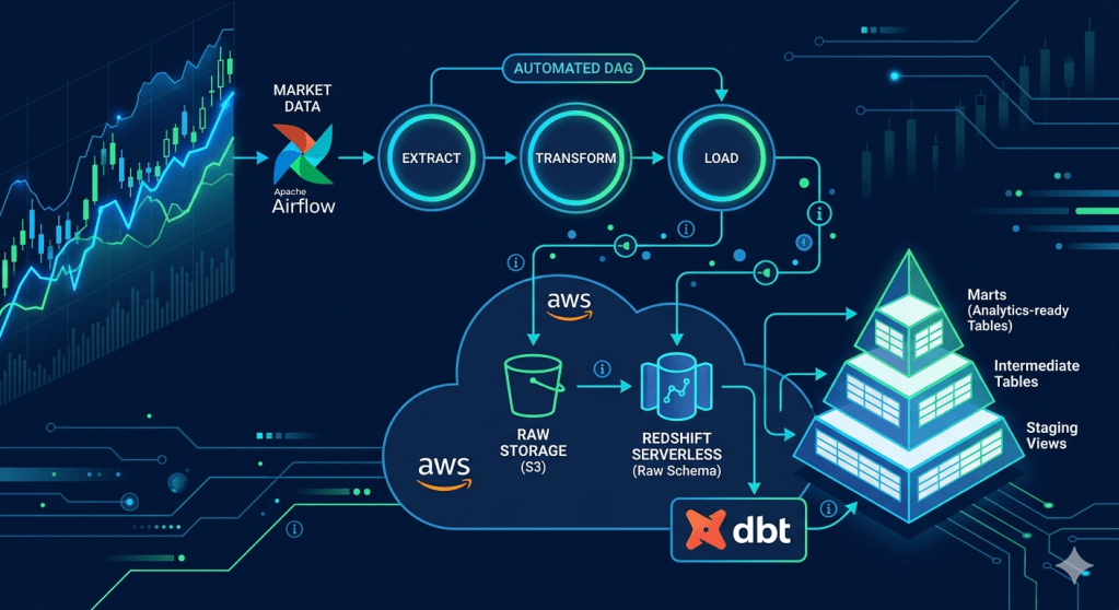
In the next part, we’ll bring in Apache Airflow to replace the manual pipeline execution, and dbt to transform our raw Redshift tables into analytics-ready models with proper lineage, testing, and documentation. The pipeline is going to start looking a lot more like what you’d find in a real data team.
Stay tuned — and as always, the full code is available in this GitHub Repository


Leave a comment