
Nowadays, we can see new AI products released on a weekly basis thanks to rapidly increasing of the foundation models. However, it needs a quality data infrastructure running under the hood. Unlike README.md in the GitHub repo, which focuses on cloning the projects, this blog post explains how to build the project from scratch as a guideline for anyone getting into Data Engineering in professional environments, as much as possible. So, let’s get started.
- Project Architecture
- Tech Stack, Prerequisites, and Project Structures
- Key Design Features
- How the project was built
- Conclusion
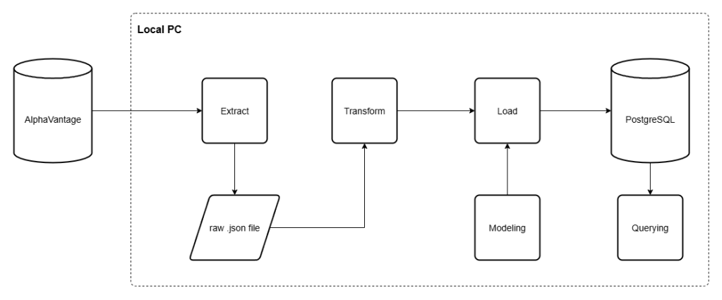
Project Architecture
At this point, this project focuses on building the ETL pipeline using the public API from AlphaVantage. With the extraction process, we will get the API response in the form of JSON, and we store it in a local machine accordingly. Then, transforming and load that data into a local PostgreSQL database. We also add ‘Modeling’ layer to add the new database table in case we created the new one.
Tech Stack, Prerequisites, and Project Structures
Tech Stacks
Amongst the choices of tools able to used for building, we build this ETL pipeline using Python and PostgreSQL combination, as they are popular tools amongst modern Data Engineers out there. Noted that we aren’t implementing fancy AI model stuffs at this point, as we’re focusing on building the ETL pipeline as a solid foundation. We will show you how to use those fancy tools later in the following projects.
| Layer | Tools used |
| Language | Python 3.9+ |
| Database | PostgreSQL 15 |
| Database Driver | psycopg2-binary |
| Database Toolkit | SQLAlchemy |
| Data Processing Library | pandas |
| HTTP | requests |
| Configuration | python-dotenv |
| Containerization | Docker |
| Testing | pytest |
Prerequisites
- Python 3.9 or later
- Docker Desktop (for hosting and running PostgreSQL container)
- AlphaVantageAPI (you could sign up for a free API key here)
AlphaVantage is a financial data services provider that also offers a public API to access their data. Not only OHLCV (Open, High, Low, Close, Volume) data, but also the financial reports, and other useful financial information for developers to work with.
With the free-tier API keys, we could make a request 5 times per minute and 25 requests daily. Our project was built considering these limitations. However, in the scale of production, we could purchase the premium API keys with more relaxed limitations later.
Project Structure
In this part, our finalized project directory would look like this. We will explain about each part of them in the following section of this blog.
finance_data_platform/├── docker-compose.yml├── requirements.txt├── .env.example│├── sql/│ └── sma.sql # Calculate SMA5 and SMA20│ └── daily_returns.sql # Calculate daily returns│ └── volatility.sql # Calculate volatility (standard deviation) of the returns from last 21 trading days│ └── cumulative_return.sql # Calculate cumulative returns of the stocks from the earliest OHLCV data of stocks│├── data/│ ├── raw/{symbol}/ # Raw JSON responses from AlphaVantage│ └── analytics/ # Extracted files for SQL query│├── src/│ ├── db_connect.py # psycopg2 connection factory (reads from .env)│ ├── pipeline.py # Main ETL orchestration (fetch → transform → load)│ ├── reprocess_pipeline.py # Load from local files without API calls│ ├── analytics.py # Save the SQL query into .csv file│ ││ ├── extract/│ │ └── alphavantage_ingest.py # API fetch with rate-limit retry and quota detection│ ││ ├── transform/│ │ └── transform_stock.py # OHLCV + calendar attribute derivation; metadata parsing│ ││ ├── load/│ │ ├── dimension_loader.py # Bulk-insert dim_date and dim_metadata (ON CONFLICT DO NOTHING)│ │ └── fact_loader.py # Bulk-insert stock_prices; get_max_loaded_date for incremental load│ ││ └── modeling/│ ├── create_dimension_tables.py│ ├── create_fact_tables.py│ └── create_indexes.py│└── tests/ ├── conftest.py # db_cursor fixture — isolated TEMP tables per test ├── test_transform.py # Unit tests for transformation logic └── test_loaders.py # Integration tests for all loaders (dim + fact)
Key Design Features
- Batch ETL Pilelines: Fetch, Transform, and Load financial data
- Star Schema: Dimensional modeling for analytical queries
- Error Handling: API rate limit handling, database error rollback
- Containerization: With both SQL container (run by Docker) and a virtual environment, this project could run on almost any machine
- Testing: Unit tests for critical data transformation logic
- Transaction Safety: Atomic operations with rollback on failure
- Single transaction per symbol: both dimention and fact table shared a single connection commit, make it more safe for orphaned dimentions without corresponding facts.
- Idempotent writes: all inserted statements use
ON CONFLICT DO NOTHING, make it safe to re-run. - Incremental loading:
get_max_loaded_date()prevents re-inserting existing OHLCV data into database, keeping loading efficient after the initial backfill. - Bulk inserts: when possible, we implement bulk loading process into the database significantly reduce processing time of loading row-by-row.
- Test isolation: we design the testing mechanism to work with temporary tables to test the connection and ETL logics, isolate the testing data from the real ones.
How the project was built
Setting up the project
Create and initialize a PostgreSQL container with Docker
First, we need to create the PostgreSQL Docker container to run the SQL virtually without actually installing it into the local machine. No need to be concerned about the local machine’s dependencies.
To do so, we create the docker-compose.yml file first. As we need only PostgreSQL in the container, we need to define the container’s specification as follows:
# define docker versionversion: '3.8'# define services used in containerservices: postgres: image: postgres:15 container_name: finance_postgres restart: always environment: POSTGRES_USER: finance_user POSTGRES_PASSWORD: finance_password POSTGRES_DB: finance_db ports: - "5432:5432" volumes: - postgres_data:/var/lib/postgresql/datavolumes: postgres_data:
After defining the container’s specification, we need to compose it as a container using the following command in the terminal.
docker compose up -d
Then, you could verify and run your compose using the following command. Make sure that your container name is visible after you verify it. Otherwise, you need to stop the other container that uses the same port (in this case, 5432 for PostgreSQL). Then compose the container again. Finally, run the container using these terminal command.
# verify the containerdocker ps# run the containerdocker exec -it finance_postgres psql -U finance_user -d finance_db
If you do that correctly, the terminal will turn into PostgreSQL terminal, that starts with finance_db=#.
Create and configure a virtual environment
After we create the PostgreSQL container to make it run without concern of dependencies, we also need to make sure that our projects should be able to run on any machine, regardless of dependencies. To do so, we need to create VIrtual Environment for the project using the following commands.
# create venv folderpython -m venv venv# for PowerShell user, we need to set the execution policy before activating the venvSet-ExecutionPolicy -Scope CurrentUser -ExecutionPolicy Unrestricted -Force# activate the venv, for PowerShell users, we use the followings.\venv\Scripts\Activate.ps1
After we activate the virtual environment, we need to install the required Python libraries into the project using this command.
# install the required packagespip install requests pandas psycopg2-binary python-dotenv pytest# save the required packages as requirementspip freeze > requirements.txt
Save and secure your environment variables
Practically, we don’t hardcode the confidential information, like API key and SQL database information, directly into the Python scripts, as it’s exposed to unauthorized usage. We need to save it into the files that would be never committed publicly. We called it the environment (.env) file. So, create the .env file, then input the following data into it.
ALPHAVANTAGE_API_KEY=<alphavantage_api_key_here>DB_HOST=localhostDB_PORT=5432DB_NAME=finance_dbDB_USER=finance_userDB_PASSWORD=finance_password
If you’re gonna share this file publicly through a GitHub repository, make sure that you include .env file into the list of .gitignore files before committing them. Therefore, the .gitignore should at least include this item
.env
Pipeline walkthrough
Extract
In this point of this project, we’re going to extract..
- Daily OHLCV data of the specified stocks
- Metadata of stocks containing full company name, sector, industries, financial ratios, and so on.
To do so, we need to look up from the AlphaVantage API documentation to see how we could get that data. We found that we need to call for daily OHLCV data from “TIME_SERIES_DAILY” function, then get the Company’s metadata from “OVERVIEW” function.
As we’re using the free-tier API key, obviously, we also have the request limitations. At least we know that we have the limit of 5 API request per minute, and 25 requests per day. Moreover, we have the limited scope for OHLCV data as daily granularity for the last 100 days (outputsize=compact) only. So, we need to configure the fetching mechanism regarding these limitations
Here’s how the code looks like, for now:
import requestsimport osimport jsonfrom datetime import datetimeimport timeimport loggingimport pathlibfrom dotenv import load_dotenv# load environment variables from .env file to the codespaceload_dotenv()# refer API key from .env fileAPI_KEY = os.getenv('ALPHAVANTAGE_API_KEY')# define the logger object to inform the progress along the waylogger = logging.getLogger(__name__)# create the target filepath (where the fetched files are saved into)RAW_DATA_DIR = pathlib.Path(__file__).parent.parent.parent / "data" / "raw"# fetch(extract) the OHLCV datadef fetch_stock_prices(symbol): # to fetch the data, we need the querying URL url = "https://www.alphavantage.co/query" # and also the query itself. We need to use the query as dictionary as required from requests.get() method. noted that the dictionary keys must comply with API function parameters. params = { "function": "TIME_SERIES_DAILY", # function to call for daily OHLCV data "symbol": symbol, # pass the symbol from method parameters to query parameters "apikey": API_KEY, # refer the loaded API key "outputsize": "compact" # define the output size } # fetch the data, if it uses more than 60 secs for a request, kill it. response = requests.get(url, params=params, timeout=60) # in case of other responses than 200 (HTTPError), raise it response.raise_for_status() # save the response as JSON data = response.json() # AlphaVantage returns the "Information" in case that the request wasn't fulfilled e.g. attempting intraday data with free-tier API keys if "Information" in data: raise RuntimeError(f"AlphaVantage daily quota exceeded for {symbol}: {data['Information']}") # In case exceeding usage quota, AlphaVantage returns "Note" response. So we could wait and retry for a few times. if "Note" in data: for attempt in range(1, 4): logger.warning(f"API rate limit reached for {symbol}. Attempt {attempt}/3 — waiting 60 seconds...") time.sleep(60) retry_response = requests.get(url, params=params, timeout=60) retry_response.raise_for_status() retry_data = retry_response.json() if "Note" not in retry_data: data = retry_data break else: raise RuntimeError(f"API rate limit for {symbol} persisted after 3 retry attempts") # In case that request is invalid or cannot be processed, return "Error Message" if "Error Message" in data: logger.error(f"API error for {symbol}: {data['Error Message']}") raise RuntimeError(f"AlphaVantage API error for {symbol}: {data['Error Message']}") # create the timestamp for OHLCV data timestamp = datetime.utcnow().strftime("%Y-%m-%d") # create new blank .json file into target directory. If it's not existed yet, create the new one filepath = RAW_DATA_DIR / symbol / f"{symbol}_{timestamp}.json" filepath.parent.mkdir(parents=True, exist_ok=True) # write the extracted .json response into file, then save close it. with open(filepath, "w") as f: json.dump(data, f) return str(filepath)# fetch the company metadatadef fetch_company_metadata(symbol): # define URL and query parameters as in OHLCV data url = "https://www.alphavantage.co/query" params = { "function": "OVERVIEW", "symbol": symbol, "apikey": API_KEY } # fetch the response and store as data response = requests.get(url, params=params, timeout=60) response.raise_for_status() data = response.json() # Error Handling if "Information" in data: raise RuntimeError(f"AlphaVantage daily quota exceeded for {symbol} metadata: {data['Information']}") if "Note" in data: for attempt in range(1, 4): logger.warning(f"API rate limit reached fetching metadata for {symbol}. Attempt {attempt}/3 — waiting 60 seconds...") time.sleep(60) retry_response = requests.get(url, params=params, timeout=60) retry_response.raise_for_status() retry_data = retry_response.json() if "Note" not in retry_data: data = retry_data break else: raise RuntimeError(f"API rate limit for {symbol} metadata persisted after 3 retry attempts") if "Error Message" in data: raise RuntimeError(f"AlphaVantage API error for {symbol} metadata: {data['Error Message']}") # create raw .json file filepath = RAW_DATA_DIR / symbol / f"{symbol}_metadata.json" filepath.parent.mkdir(parents=True, exist_ok=True) # write the response into .json file, then close with open(filepath, "w") as f: json.dump(data, f) return str(filepath)
Transform
In transformation phase, we read the saved .json file, select the columns we need, create the new ones with calculations, and typecasting to make it comply with SQL data types. Like in the extract phase, we make a transformation on (1) OHLCV data, and (2) the Company’s metadata. We use the following instructions.
import jsonimport pandas as pd# Transform OHLCV datadef transform_stock_prices(filepath, symbol): # read the extracted JSON file with open (filepath, "r") as f: data = json.load(f) # get the dictionary values (the daily OHLCV data) from the "Time Series (Daily)" key in the JSON data >> refer to API documentation for other APIs time_series = data.get("Time Series (Daily)", {}) # {} means if the key is not found, it will return an empty dictionary instead of throwing an error # create the blank lists, we will append it in the following for loop records = [] for date, values in time_series.items(): # convert the date string to datetime object, we made it here to reduce the computations overhead than converting it in the loop dt = pd.to_datetime(date) # select the symbol, date, OHLCV data, then create the new date columns built from date records.append({ "symbol": symbol, # pass the argument symbol to the function and include it in the records "date": dt, # convert the date string to a datetime object "open": float(values["1. open"]), "high": float(values["2. high"]), "low": float(values["3. low"]), "close": float(values["4. close"]), "volume": int(values["5. volume"]), "day" : dt.day, "month" : dt.month, "year" : dt.year, "quarter" : ((dt.month - 1) // 3) + 1, # ensure the quarter is classified correctly "day_of_week" : dt.dayofweek, # Monday=0, Sunday=6 "week_of_year" : int(dt.isocalendar().week) # typecasting to int to avoid pandas Int64 type which is not compatible with psycopg2 when loading into the database }) # convert the list into the dataframe df = pd.DataFrame(records) return df# Transform company's metadatadef transform_company_metadata(filepath): with open(filepath, "r") as f: data = json.load(f) # get the dicionary values symbol = data.get("Symbol", "") if not symbol: raise ValueError(f"Metadata file is missing 'Symbol' field. The file may contain an API error response.") # this time, we store it as dictionary metadata = { "symbol": symbol, "company_name": data.get("Name", ""), "sector": data.get("Sector", "") } return metadata
You could see that we return the DataFrame for OHLCV data, but just a Python dictionary for company metadata. The reason behind them is that the OHLCV data is the multi-row tabular data, while metadata source file is just a single row data.
Modeling
Basically, the modeling process is the layer to monitor and create tables in the SQL database. It might not be required in building a classic ETL pipeline, as we could build it right into your SQL database only once, but adding the modeling layer has its own benefits, such as:
- Reproducibility across environments: In case we need to run this project on the new machine e.g. Teammate’s laptop, Docker container, or CI/CD server — the modeling layer rebuilds the schema automatically without creating the table manually in SQL terminal.
- Version control & auditability: When we made changes on a column through this layer, the change would be visible across Git commits. Leave the audit trail for future inspection.
- Orchestration: As the table was wrapped as a Python method, it’s also callable through our orchestration scripts (
pipeline.py). We place it before the loading process to ensure that the transformed data has the table in SQL database to be loaded into. Otherwise, we need to create them first. - Safe to run repeatedly: under the proper query, using
CREATE TABLE IF NOT EXISTSclause ensures that the new table would not be created unreasonably.
At t his phase of this project, we only need to create 3 SQL tables.
- OHLCV data as the fact tables
- Dates and Metadata as the dimension tables
How’s the fact table models looks like.
# borrow the connection config from db_connect.pyfrom db_connect import db_connectdef create_fact_table(): # open the SQL connection conn = db_connect() # create a cursor object to interact with the database cursor = conn.cursor() # check the SQL database if they have SQL tables. If not, create the new one. cursor.execute( """ CREATE TABLE IF NOT EXISTS stock_prices ( symbol TEXT, date DATE, open NUMERIC, high NUMERIC, low NUMERIC, close NUMERIC, volume BIGINT, PRIMARY KEY (symbol, date), FOREIGN KEY (symbol) REFERENCES dim_metadata(symbol), FOREIGN KEY (date) REFERENCES dim_date(date) ); """ ) # send the query string to SQL conn.commit() # close both cursor object and connection cursor.close() conn.close()# entry point guard to regulate execution sequence in the pipelineif __name__ == "__main__": create_fact_table()
And here’s how dimension table looks like.
from db_connect import db_connectdef create_dim_dates(): # open the SQL connection, it requires host, port, database_name, username, and password conn = db_connect() # create a cursor object to interact with the database cursor = conn.cursor() # create the dim_dates table if not exists, otherwise do nothing cursor.execute( """ CREATE TABLE IF NOT EXISTS dim_date ( date DATE PRIMARY KEY, day INT, month INT, year INT, quarter INT, day_of_week INT, week_of_year INT ); """ ) conn.commit() # commit the transaction to save changes cursor.close() # close the cursor conn.close() # close the connectiondef create_dim_metadata(): conn = db_connect() cursor = conn.cursor() cursor.execute( """ CREATE TABLE IF NOT EXISTS dim_metadata ( symbol TEXT PRIMARY KEY, company_name TEXT, sector TEXT ); """ ) conn.commit() # cursor.close() conn.close()# entry point guardif __name__ == "__main__": create_dim_dates() create_dim_metadata()
Load
After we ensure that the fetched data is cleaned into the format we need (transform) and we have the proper table to load it into (modeling), the next step is to load the transformed data into the modeled SQL tables.
Here we also have the fact loader for OHLCV data and dimension data for dates and metadata, like the prior steps.
Before loading data right into SQL, we need to ensure that the loaded data is not duplicated in the existing SQL tables. In this case, we are talking about OHLCV data, which is designed to fetch the historical 100 days of data, so the data inside the SQL table would be 100x redundant without proper regulation.
Here’s how we created the loading logic for fact tables. Noted that we use get_max_loaded_date() method to find out the latest loaded date of each stock into the database. When we get those dates, we will compare the transformed data to find the incremental data that needs to be loaded. You’ll see how it works in the orchestration phase of this pipeline.
from psycopg2.extras import execute_valuesimport logginglogger = logging.getLogger(__name__)# open the connection to the PostgreSQL database using credentials from environment variablesdef load_stock_prices(cursor, df): # insert data into stock_prices table as a bulk # Convert all numpy types to Python native types to avoid psycopg2 adapter errors fact_columns = ["symbol", "date", "open", "high", "low", "close", "volume"] # select the columns df_copy = df[fact_columns].copy() # create a copy with selected columns to avoid modifying the original DataFrame df_copy['date'] = df_copy['date'].dt.to_pydatetime() # numpy.datetime64 -> datetime # Use .values.tolist() to convert numpy types to native Python types values = [tuple(row) for row in df_copy[fact_columns].values.tolist()] # write the query to load the transformed values to SQL table insert_query = """ INSERT INTO stock_prices (symbol, date, open, high, low, close, volume) VALUES %s ON CONFLICT (symbol, date) DO NOTHING """ # load the value into table as a bulk execute_values(cursor, insert_query, values) logger.info(f"Loaded {len(values)} new rows into stock_prices")def get_max_loaded_date(cursor, symbol): """ Check for the latest date loaded for each symbol in fact table. """ cursor.execute( "SELECT MAX(date) FROM stock_prices WHERE symbol = %s;", (symbol,) ) # fetchone() returns a tuple, we want the first element which is the max date result = cursor.fetchone() max_date = result[0] logger.info(f"Latest loaded date for {symbol}: {max_date}") return max_date
And this one for dimension tables:
from psycopg2.extras import execute_valuesimport logging# create logging object to return the execution log to userlogger = logging.getLogger(__name__)def load_dim_dates(cursor, df): """ Load the date dimensions in bulk, reduce the load time significantly than the iteration row-by-row """ date_cols = ['date', 'day', 'month', 'year', 'quarter', 'day_of_week', 'week_of_year'] df = df[date_cols].drop_duplicates() values = [tuple(row) for row in df.values.tolist()] # convert each low to the list of tuples so it could be loaded as a bulk insert_query = """ INSERT INTO dim_date (date, day, month, year, quarter, day_of_week, week_of_year) values %s ON CONFLICT (date) DO NOTHING; """ # load values as a bulk into SQL tables execute_values(cursor, insert_query,values) logger.info(f"Loaded {len(values)} rows into dim_date")def load_dim_metadata(cursor, metadata): # insert one row (metadata) into SQL metadata table cursor.execute( """ INSERT INTO dim_metadata (symbol, company_name, sector) VALUES (%s, %s, %s) ON CONFLICT (symbol) DO NOTHING; """, (metadata["symbol"], metadata["company_name"], metadata["sector"]) ) logger.info(f"Loaded metadata for {metadata['symbol']} into dim_metadata")
Orchestrate the Pipeline
Finally, we will orchestrate those created methods to make them works together in the defined sequences. Here’s how we designed the orchestration processes:
- Create the fact and dimension table for OHLCV and metadata, respectively.
Then, for each selected stocks, we orchestrate ETL pipeline with the following process.
- Fetch OHLCV and metadata from AlphaVantage with free-tier API. We let the code sleep for 12 secs after each API request to make it comply with the minute-wise free-tier requests (5 requests per minute)
- Transform OHLCV and metadata into the desired form
- Look up the latest data we have in the SQL table, create a filter to load only the data point occurred from that date.
- Load both OHLCV and metadata of the stock into SQL table.
For each process, we mount the logging process to leave a trail for users when something goes wrong.
Here’s how the orchestration process looks like:
import loggingimport timefrom db_connect import db_connectfrom extract.alphavantage_ingest import fetch_stock_prices, fetch_company_metadatafrom transform.transform_stock import transform_stock_prices, transform_company_metadatafrom load.fact_loader import load_stock_prices, get_max_loaded_datefrom load.dimension_loader import load_dim_dates, load_dim_metadatafrom modeling.create_dimension_tables import create_dim_dates, create_dim_metadatafrom modeling.create_fact_tables import create_fact_tablefrom modeling.create_indexes import create_indexes# config the logging to display info level messages with timestampslogging.basicConfig( level=logging.INFO, format = '%(asctime)s - %(name)s - %(levelname)s - %(message)s', datefmt = '%Y-%m-%d %H:%M:%S')logger = logging.getLogger(__name__)def run(symbols): # build up the connection with the borrowed scripts from cb_connect.py conn = db_connect() cursor = conn.cursor() # create a cursor object to interact with the database for symbol in symbols: try: # fetch the data from the API, we use 12 secs sleep after each API call to respect free tier limit (5 calls per minute) logger.info(f"Fetching {symbol}") filepath = fetch_stock_prices(symbol) time.sleep(12) metadata_filepath = fetch_company_metadata(symbol) time.sleep(12) # transform the data and metadata logger.info("Transforming") df = transform_stock_prices(filepath, symbol) metadata = transform_company_metadata(metadata_filepath) # add the incremental loading logic here by checking the max date already loaded for the symbol in the fact table max_date = get_max_loaded_date(cursor, symbol) if max_date is not None: df = df[df["date"].dt.date > max_date] # filter the dataframe to only include rows with date greater than max_date logger.info(f"{symbol}: {len(df)} new rows after {max_date}") if df.empty: logger.info(f"{symbol}: no new data to load, skipping") continue # load the dimension tables first, as the fact table has foreign key associated to them logger.info("Populating dimension tables") load_dim_dates(cursor, df) load_dim_metadata(cursor, metadata) # load the fact table with transformed data logger.info("Loading into fact table") load_stock_prices(cursor, df) conn.commit() # in case anything goes wrong for each stocks, we cancelled out the commit for that stock, then raise an error except Exception as e: conn.rollback() logger.error(f"Pipeline failed: {e}") raise# Orchestrate all processes togetherif __name__ == "__main__": symbols = ["NVDA","AAPL","MSFT","GOOGL","AMZN"] create_dim_dates() # ensure the dim_dates table is created before loading data create_dim_metadata() # ensure the dim_metadata table is created before loading data create_fact_table() # ensure the fact table is created before loading data create_indexes() # create indexes on the fact table for performance run(symbols)
Testing the pipeline
There’s no proper ETL pipeline without proper testing. So, we create testing package for this project. This is how we do it:
After we create a /tests folder, we create __init__.py which is basically the blank file. Doing so lets the machine treat the /tests folder as a package, which could be managed and run with more ease and resilience. Even though it isn’t required in modern pytest (ver 3.0+) anymore, but __init__.py is still required for pytest.ini or pyproject.toml, which are the common workflow configurations in modern days.
Then, we set the conftest.py to configure the test scope (in this case, integration test), and store the test fixture with the decorator @pytest.fixture for further integration tests. Here’s how it looks like:
import pytestimport psycopg2from src.db_connect import db_connect# scope the integration test. We will mention it in the integration test, and we could also scope only the integration test later in the terminal.def pytest_configure(config): config.addinivalue_line( "markers", "integration: mark a test as an integration test that requiring a live PostgreSQL connection (docker compose up -d)" )# set the figure, we would use it now and later when the test loaders need the tablepytest.fixture(scope="function")def db_cursor(): """ Connect to the real Postgres instance and create TEMP tables , which mimics the production schema. Each test gets a clean slate; connection is rolled back and closed after the test regardless of pass/fail. Skip automatically if Postgres is not reachable. """ try: conn = db_connect() except psycopg2.OperationalError: pytest.skip("PostgreSQL is not reachable, compose the docker container first via: docker compose up -d") conn.autocommit = False cursor = conn.cursor() """ TEMP tables are session-scoped and don't support cross-table foreign keys (FK) constraints, so they are defined without them here. They are auto-dropped when the connection is closed . """ # create temp date dimension table cursor.execute( """ CREATE TEMP TABLE dim_date ( date DATE PRIMARY KEY, day INT, month INT, year INT, quarter INT, day_of_week INT, week_of_year INT ); """ ) # create temp metadata dimension table cursor.execute( """ CREATE TEMP TABLE dim_metadata ( symbol TEXT PRIMARY KEY, company_name TEXT, sector TEXT ); """ ) # create temp fact table cursor.execute( """ CREATE TEMP TABLE stock_prices ( symbol TEXT, date DATE, open NUMERIC, high NUMERIC, low NUMERIC, close NUMERIC, volume BIGINT, PRIMARY KEY (symbol, date) ); """ ) yield cursor # yield the cursor to the test function. This was used to separate the setup and teardown logic, which is a best practice for test fixtures. conn.rollback() # rollback any changes to ensure test isolation cursor.close() conn.close()
Then, we’ll conduct the test on the transform and load process in test_transform.py and test_loaders.py, respectively. You could see the full tests in this GitHub repository, but we could show you briefly how it works.
In transformation testing, we build up the class for each transformation component (OHLCV, metadata), then the edge cases. We define the mockup row as a fixture, then process it through actual transformation function and assure the results as we need. Here’s how it looks like, for example:
import pytestimport pandas as pdfrom datetime import datetimeimport jsonimport tempfileimport osfrom src.transform.transform_stock import transform_stock_prices, transform_company_metadataclass TestTransformStockPrices: ...class TestTransformCompanyMetadata: pytest.fixture def sample_metadata_response(self): """ Create a mock metadata API response to interact with the following testing methods. """ return { "Symbol": "AAPL", "Name": "Apple Inc.", "Sector": "Technology", "Industry": "Consumer Electronics" } def test_transform_metadata_returns_dict(self, sample_metadata_response): """ Ensure that transformed data is a dictionary. """ with tempfile.NamedTemporaryFile(mode="w", suffix=".json", delete=False) as f: json.dump(sample_metadata_response, f) temp_filepath = f.name try: result = transform_company_metadata(temp_filepath) assert isinstance(result, dict) finally: os.unlink(temp_filepath)
As the transformation phase doesn’t require communication with containerized SQL, we could call it the ‘unit test’. The next process is testing on the load phase, which needs to communicate with Docker (PostgreSQL), as we need to ensure the data migration process from local Python codespaces to SQL database is working smoothly, we also call this the ‘integration test’ and that’s what the configuration in conftest.py comes in handy here. We use the similar structure to conduct the test, but we have to use the decorator @pytest.mark.integration over the class to declare that it’s the integration tests. Here’s how it looks like for example:
import pytestimport pandas as pdfrom datetime import datefrom src.load.fact_loader import load_stock_prices, get_max_loaded_datefrom src.looad.dimension_loader import load_dim_dates, load_dim_metadata# define the helper functions for further testing as show belowdef _dim_date_row(date_str): dt = pd.Timestamp(date_str) return { "date": dt, "day": dt.day, "month": dt.month, "year": dt.year, "quarter": ((dt.month - 1) // 3) + 1, "day_of_week": dt.dayofweek, "week_of_year": int(dt.isocalendar().week) } def _price_row(symbol, date_str, opening=148.0, closing=150.0): dt = pd.Timestamp(date_str) return { "symbol": symbol, "date": dt, "open": opening, "high": closing + 1, "low": opening - 1, "close": closing, "volume": 25000000, "day": dt.day, "month": dt.month, "year": dt.year, "quarter": ((dt.month - 1) // 3) + 1, "day_of_week": dt.dayofweek, "week_of_year": int(dt.isocalendar().week) }# create the class of testing methodspytest.mark.integrationclass TestLoadDimDates: ...pytest.mark.integrationclass TestLoadStockPrices: def _seed(self, db_cursor, dates=("2026-03-09", "2026-03-08"), symbol="AAPL"): """ Helper method to seed the dim_date and dim_metadata tables with the necessary data for testing the fact loader. """ dim_df = pd.DataFrame([_dim_date_row(d) for d in dates]) load_dim_dates(db_cursor, dim_df) load_dim_metadata(db_cursor, {"symbol": symbol, "company_name": "Apple Inc.", "sector": "TECHNOLOGY"}) def test_inserts_rows(self, db_cursor): """ Given the blank stock_prices fact table, when we load a stock price record, then it should be inserted into the table in just one row. """ self._seed(db_cursor) df = pd.DataFrame([_price_row("AAPL", "2026-03-09"), _price_row("AAPL", "2026-03-08")]) load_stock_prices(db_cursor, df) db_cursor.execute("SELECT COUNT(*) FROM stock_prices;") assert db_cursor.fetchone()[0] == 2
The integration tests work with the temporary table as defined in conftest.py then use the actual loaders method to load the mockup data into the temporary table, then drop those tables safely to ensure that this mockup data wouldn’t loaded into the production tables.
Finally, the full flow of pytest could be illustrated as follows:
pytest ├── discovers tests/conftest.py → registers "integration" marker ├── test_transform.py (unit tests) │ └── no db_cursor → runs immediately, no Docker needed └── test_loaders.py (integration tests) └── requests db_cursor fixture ├── tries db_connect() ├── if Docker is down → pytest.skip() └── if Docker is up → creates TEMP tables → yields cursor → test runs → rollback → cleanup
Then, we run the test using the following command:
# use this one to run everythingpytest tests/ -v# use this one to only run on the integration tests# make sure the docker PostgreSQL container is running. Otherwise run docker compose up -dpytest tests/ -v -m integration
Querying the pipeline
After we pass all tests, we can ensure that the ETL pipelines work properly from API fetching to loading into SQL. In the next phase, we would use SQL queries to extract the loaded data into .csv files.
First, we build up the SQL queries under the folder /sql. Each .sql file contains a different query for maintainability purposes. For example, we calculate the daily return using the following query:
SELECT s.symbol, s.date, s.close, LAG(s.close) OVER ( PARTITION BY s.symbol ORDER BY s.date ASC ) AS prev_close, ROUND ( (s.close / LAG(s.close) OVER ( PARTITION BY s.symbol ORDER BY s.date ASC)) - 1, 4 ) AS daily_return FROM stock_prices sORDER BY s.symbol, s.date ASC;
When we create all queries (we have 4 queries at this point — SMA, daily returns, volatility, and cumulative returns), we will orchestrate the query process which have the following steps:
Create Engine with SQL connection string → Lookup the queries → Create output directory → Read the query and export the results → Dispose the engine
We orchestrate the querying process in /src/analytics.py as detailed as follows:
import pandas as pdfrom pathlib import Pathfrom db_connect import db_connectimport loggingfrom sqlalchemy import create_enginefrom dotenv import load_dotenvimport osload_dotenv()logger = logging.getLogger(__name__)# create SQLAlchemy engine for database connection using connection stringengine = create_engine( f"postgresql+psycopg2://{os.getenv('DB_USER')}:{os.getenv('DB_PASSWORD')}@{os.getenv('DB_HOST')}:{os.getenv('DB_PORT')}/{os.getenv('DB_NAME')}")# lookup the queries from /sqlQUERIES = { "sma": Path("sql/sma.sql"), "daily_returns": Path("sql/daily_returns.sql"), "volatility": Path("sql/volatility.sql"), "cumulative_return": Path("sql/cumulative_return.sql")}# create output directory to save the analytics resultsOUTPUT_DIR = Path("data/analytics")OUTPUT_DIR.mkdir(parents=True, exist_ok=True)# connect to the database and execute each query, saving the results as CSV filesconn = db_connect()# execute each query and save the results to CSV filesfor name, sql_path in QUERIES.items(): query = sql_path.read_text() df = pd.read_sql_query(query, conn) output = OUTPUT_DIR / f"{name}.csv" df.to_csv(output, index=False) logger.info(f"Exported {name} to {output}")# close the database connectionengine.dispose()
Conclusion
At this point, we create the classic ETL pipeline, starting from fetching data from external sources with public API keys, transforming the data into the format we need, and then loading it into a local SQL database. Moreover, we create and manage the SQL schema through the modeling phase for reproducibility across environments and version control. After that, we conduct the testing procedures to ensure that the transformation unit and database integration work properly. After that, we create the analytics layer to fetch data from the SQL database, do some calculations through SQL queries, and then save the results into .csv files. To make this project executable across environments, we built this project under virtual environments and a containerized SQL database.
In the next part, we will move forward from building the local ETL pipeline to cloud using AWS services. Stay tuned.


Leave a comment