Data analysis and predictions of Diabetes

Diabetes become one of the fourmain non-communicable diseases (NCD) – besides of Cardiovascular Disease, Cancer, and Chronic respiratory.

In accordance with information from World Health Organization (WHO), around 14% of all adults worldwide suffer the diabetes. Moreover, many of them were not covered by proper medical treatment, especially in low and middle income coutries.

This analysis takes you through actual survey obtained from people across US, we will explore the datasets, and how we apply the actual data analysis and predictions mechanism onto it.

This project is showcase how we obtain and transform the real-world datasets. Then, illustrate how we implement exploratory data analysis and machine learning methodologies onto the datasets.

Data source

We use the ‘Behavioral Risk Factors Surveillance Systems’, which is the Survey conducted annually by the United States’ Center of Disease Control. You could access our sources used here.

After we download the source as .xpt file, we could use pandas library to load the files into our workspace using python script as follows.

# import libraries
import pandas as pd

# import data
raw_data = pd.read_sas('LLCP2023.XPT', format='xport')

# examine first few rows of the data
raw_data.head()

Understand the data

The raw data itselfs has 350 columns, contains the survey results from people across US regarding their health conditions, and relevant daily behaviors, such as physical and mental health conditions, physical activity, smoking, drinking behaviors, and existing chronic diseases.

These data could be obtained from the files called codebook, which explains the values in each column thoroughly.

Amongst those number of columns, we extract just some of them (around 25 – 30) which considered to be relevant to diabetes such as BMI (Body Mass Index), Self-assess general health conditions, Age, and existing chronic diseases including diabetes itself. We will use the known diabetes for analysis and predictions procedure.

[Editor’s note: we could adapt BRFSS survey for development to other chronic diseases predictions e.g. high blood pressure, asthma, etc., which depends on availability of relevant attributes.]

After we selected those columns, we need to transform some of them, which we could use the procedure as follows.

Fill the missing values (“NaN”)and nonregular values (77, 88, and 99) values of ‘AVEDRINK3’ columns with 0, assumed that those are non-drinkers.
Drop ALL missing vlaues from the selected columns.
With and existing rows, we need to go through each columns, then do either drop, replace, or recalculate the values, or all of them. We use the following python syntax to do those process:

# replace the value
data['COLUMN'] = data['COLUMN'].replace({old_value:new_value})

# drop the row with particular value
data.drop(data[data['COLUMN'] == drop_value].index, inplace=True)

You could see the full details from the source code here.
Export the cleaned datasets as seperated .csv files for further visulization work.

Data Exploration

After the extraction and transformation of the data, we could go through the data exploration, which we visualize it through PowerBI. We could see the overview of the dataset as shown in the list below:

Portion of People with known diabetes

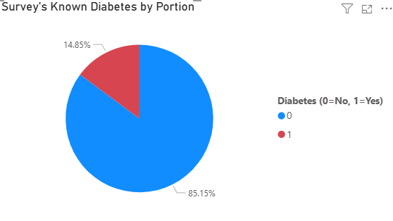
As you can see that the survey shows that samples from BRFSS–which is solely conducted in the US–have portion of samples with known diabetes by 14% approximately. Aligned with claims from WHO.
Known diabetes by Body Mass Index (BMI)

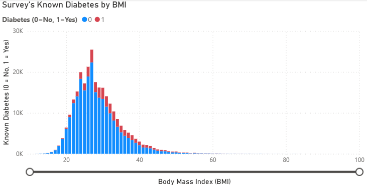
We plot the count of known diabetes with distribution of Body Mass Index (BMI) and found something interesting that.
- Higher the respondent’s BMI, higher the portion of Known diabetes response.
- There’s around 3% of all respondant with oddly high BMI. We considered that those oddly high BMI is possible in some people. As this value is calculated from Hight and Weight which is quite common matrices, and we believe that BMI play the significant role for Diabetes prediction. So, we decide to include this factor into our Prediction using Machine Learning Algorithm.
Known Diabetes portion by Age grouup
As we explore the data, we found some relationship between konwn diabetes with the respondent’s age. To be said, around 10% of people in late 40s faced diabetes, and higher then.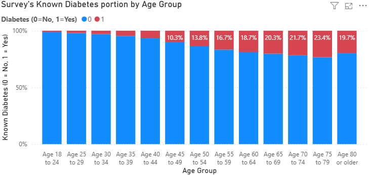

Diabetes Prediction

In this part, we will illustrate how we develop the diabetes predictions model using statistical and machine learning procedures.

Behavioral Risk Factors Correlation to Diabetes

We will apply.corr() method acrossd all columns we selected into the datasets, then plotted them into matrix form, we could see the illustration as shown below.

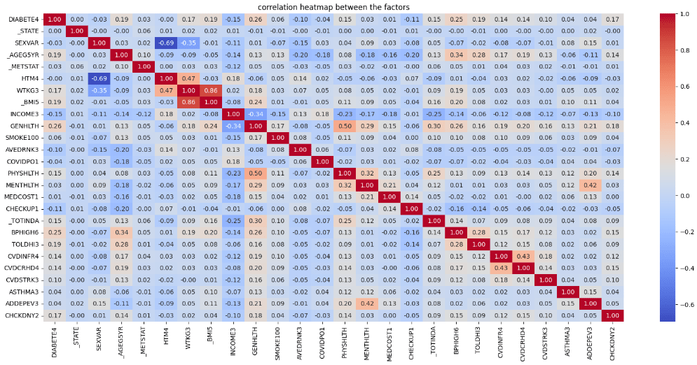
From this chart, we focused on the correlation between known diabetes (‘DIABETE4’) with other selected factors. We judgementally select 5 factors with highest absolute correlation coefficient value using the simple syntax as follows:

# select 5 attributes with highest correlation
top5 = list(data.corr()['DIABETE4'].abs().sort_values(ascending=False)[1:6])

Then, we could see that 5 attributes with the highest absolute value of correlation with known diabetes are;

GENHLTH (Self-assessed general health conditions)
BPHIGH6 (Known high blood pressure)
_BMI5 (Calculated body mass index)
TOLDHI3 (Known high Cholesterol level)
_AGE5YR (Age groups)

Then, we save it as list type variables for using it later.

Data Balancing

From the exploratory data analysis procedure, we found the imblance in number between the class of those who have diabetes, and those who doesn’t. This class imbalance may cause the inaccuracy in our prediction model. So we need to balance the datasets as follows:

# balance the data by smapling the non-diabetes person
nondiabetes_sampling = data[data['DIABETE4'] == 0].sample(len(data[data['DIABETE4'] == 1]), random_state=0)
data_balanced = pd.concat([data[data['DIABETE4'] == 1], nondiabetes_sampling])

Briefly explained, the piece of code show below is undersmapling approach to make a random samples on those who doesn’t have diabetes to have the same number of observations to those who have diabetes. Then concatenate each other into the new datasets called ‘balanced dataset’.

Predict the Diabetes

After we make up the balanced data, we will predict the diabetes using the attributes and datasets previously prepared using machine learning tools as we need to import the following libraries as shown below. Then we need to perform the process explained below.

# import ML-related libraries
import scipy
from pandas.plotting import scatter_matrix
from sklearn.model_selection import train_test_split
from sklearn.model_selection import cross_val_score
from sklearn.model_selection import StratifiedKFold
from sklearn.metrics import classification_report
from sklearn.metrics import confusion_matrix
from sklearn.metrics import accuracy_score
from sklearn.linear_model import LogisticRegression
from sklearn.tree import DecisionTreeClassifier
from sklearn.neighbors import KNeighborsClassifier
from sklearn.discriminant_analysis import LinearDiscriminantAnalysis
from sklearn.naive_bayes import GaussianNB

Select the Machine Learning Model

First things first, since we need to build up the ML model to predict if one has diabetes or not, we need to use the ML model for classification problem. In the world of ML we currently have a list of them – Logistic Regression, Linear Discriminant Analysis, K-Neighbor Classifier, Decision Tree Clasifier, and Gaussian NB. We will compare the accuracy between each model using the below code:

# select the models to compare
models = [('LR', LogisticRegression(solver='liblinear')),
('LDA', LinearDiscriminantAnalysis()),
('KNN', KNeighborsClassifier()),
('CART', DecisionTreeClassifier()),]

# create the loop to test each model and stored it for further visualization
results = []
names = []
for name, model in models:
    kfold = StratifiedKFold(n_splits = 10)
    cv_results = cross_val_score(model, x_train, y_train, cv = kfold, scoring='accuracy')
    results.append(cv_results)
    names.append(name)
    print(f"{name}: {'{:.4f}'.format(cv_results.mean())} ({'{:.4f}'.format(cv_results.std())})")

# create boxplot to compare accuracy of each model
plt.boxplot(results, labels=names)
plt.title('Accuracy Comparison by ML model')
plt.show()

Then we got the plotting results as follows:

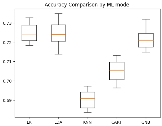
With accuracy of 72.19% , we can conclude that Logistic Regression model give us the highest accuracy for this case./head

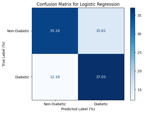
Model Optimization

After we select the Model to work on. We try to optimize the model’s accuracy through fine-tuning each parameters to see if there’s satisfactory improvement in Accuracy. Amongst the numbers of parameters provided, we optimize our Machine Learning model through these following attributes

C (Inverse of Regularization Strength) which the lower values could lower the risk of overfitting (also increse the risk of underfitting), and vice versa. In this case we try to apply [0.01, 0.1, 1, 10, 100] onto the optimization model.
max_iter (max number of iteration) indicates the maximum number of iterations. Larger the number tends to bring up with model with more accuracy. But consumed computation resources too. In this case, we will try using max iteration by 100, 300, 500, 700, and 900 iterations.
Solver (optimization algorithm) means the logic used in our logistic regression model. As of now, scikit-learn provides 3 algorithms for us–“lbfgs”, “liblinear”, and “saga”.
penalty (regularization type) means the underlying logic used in our regression method which we apply [‘l1’, ‘l2’] into our model.

After we define those parameters to be tuned, we crate a for loop to buiuld up the model using each combination of mentioned parameter value, then store and accuracucy onto new .csv files to see the results.

After the optimization, we could achieve a bit better accuracy. We could illustrate our model’s accuracy using confusion matrix as shown below.

Conclusion

Based on this survey, we are able to define that High Blood Pressure, High Cholesterol Level, Higher BMI, Aging, and General Health Conditions has the correlation with the diabetes so we could use that for our prediction using machine learning mechanism. The output itself might not be satisfied in some field of research, but we believe that this research is still useful for personal in case to identify the risk exposed to diabetes.

You could access the project’s source file here

Nextstep Analytics